Statistics of Averages from Molecular Dynamics Trajectories: Time Auto-correlation Function

DISCLAIMER: The content in this article is for demonstration purposes only and may contain errors and technical inaccuracies.

This article briefly discusses the theory behind calculating correlation time and error from molecular dynamics (MD) simulation trajectories. This article mainly refers to the following sources:

1. Principles of Modern Molecular Simulation Methods Course materials from Professor M. Scott Shell at UC Santa Barbara

Average Properties from MD Trajectories

Consider an observable variable $A$ (an example: coordinates) from MD trajectory for which we want to compute average values. The average value is given by:

\[\overline{A} = \frac{1}{n} \sum_{i=1}^{n} A_i\]

$n$ is the total number of frames in the trajectory, and $A_i$ is the value of the $A$ at the $i^{th}$ frame.

This expression can be rewritten in terms of integrals and time as:

\[\overline{A} = \frac{1}{t_{tot}} \int_{0}^{t_{tot}} A(t) dt\]

where $t$ is a given time and $A(t)$ is the value of the property $A$ at time $t$. The $t_{tot}$ is the total simulation time.

The scenario mentioned above could introduce errors to the evaluated average for the variable compared to the real scenario. This is simply because the simulation time is not long enough, or the simulation is not in equilibrium. In an ideal situation, the real average value of the variable $A$ is given by (following ergodic hypothesis):

\[\langle{A}\rangle = \lim_{t_{tot} \to \infty} \frac{1}{t_{tot}} \int_{0}^{t_{tot}} A(t) dt\]

And the corresponding variance associated with the real ensemble average is given by:

\[\sigma_{\overline{A}}^2 = \langle(\overline{A} - \langle{A}\rangle)^2 \rangle\]

As the simulation time increases (or at the limit of ${t_{tot} \to \infty}$), the variance associated with the real ensemble average should approach zero. Another important feature of such ensemble averages is that they are time-independent. This means that the ensemble average of the variable $A$ at a time $\tau$ is the same as the ensemble average of the variable $A$ at time $\tau + t$. However, this is not the case for the average values computed from MD trajectories. Within that context, a time autocorrelation function can be defined to quantify the correlation between the variable $A$ at time $\tau$ and $\tau + t$.

Time Auto-correlation Function for the Variable $A$

The time autocorrelation function for the variable $A$ is defined as:

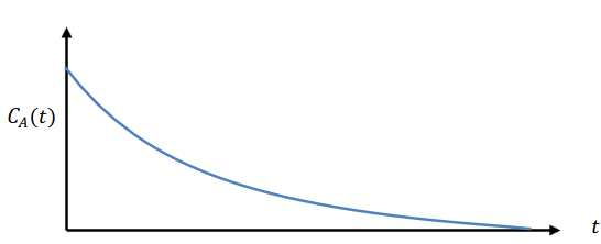
\[C_A(t) = \frac{\langle A(t+\tau) A(\tau) \rangle - \langle A(\tau) \rangle^2}{\langle A(\tau)^2 \rangle - \langle A(\tau) \rangle^2}\]

The time autocorrelation function is a measure of the correlation between the variable $A$ at time $\tau$ and $\tau + t$. As per this definition, the time autocorrelation function is normalized to 1 at $t=0$, and as the simulation time increases (or the limit of ${t_{tot} \to \infty}$), the time autocorrelation function should approach zero.

Schematically, the time autocorrelation function can be represented as the figure below, with the x-axis running from $\tau$ to $\infty$ and the y-axis running from 0 to 1:

Auto-correlation Time for the Variable $A$

The time autocorrelation function can be used to compute the correlation time for the variable $A$. The correlation time for the variable $A$ is defined as:

\[\tau_A = \int_{0}^{\infty} C_A(t+\tau) dt\]

The correlation time is a measure of the time it takes for the variable $A$ to decorrelate. The correlation time can be used to compute the error associated with the average value of the variable $A$ computed from MD trajectories.

Remarks

As mentioned above, these correlation functions and their Fourier transforms, the spectral densities, can be obtained from MD trajectories. This could provide a way to study the dynamics associated with these molecules. One particular example will be probing spherical polar coordinates of the N-H bond vector in a protein backbone (values of variable $A$ from MD trajectory frames). In this case of dipolar relaxation, the NMR relaxation parameters can be obtained from the spectral densities. The spectral densities. A future post will discuss more information about obtaining NMR relaxation parameters from MD trajectories and some CHARMM script examples.